Data

Raw and interpreted data, ready for machine learning

A model is only as good as the data behind it. GeoXMate brings every subsurface data type into one project, converts it to the project's units, and adds the interpreted products that make it useful for training.

Data import

What you can bring into a project

Each import shows what it found before anything is written, so mismatched curves, duplicate wells and unit problems are resolved at the door rather than discovered during training.

Wells with their headers, logs, deviation surveys and formation tops
3D seismic cubes in time or depth
Horizon and fault interpretations from the main interpretation packages
Maps and complete geological models with their properties

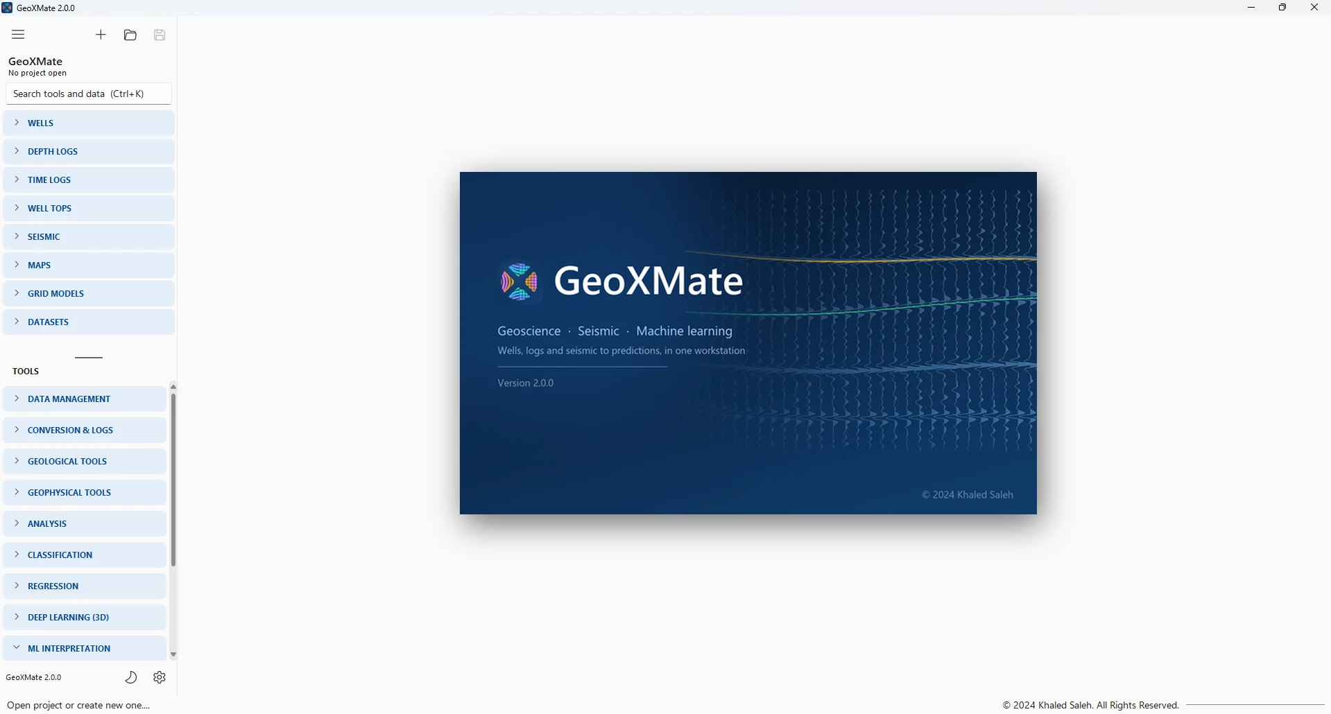
GeoXMate at launch: the project's data on the left, and the tools grouped by workflow stage below it.

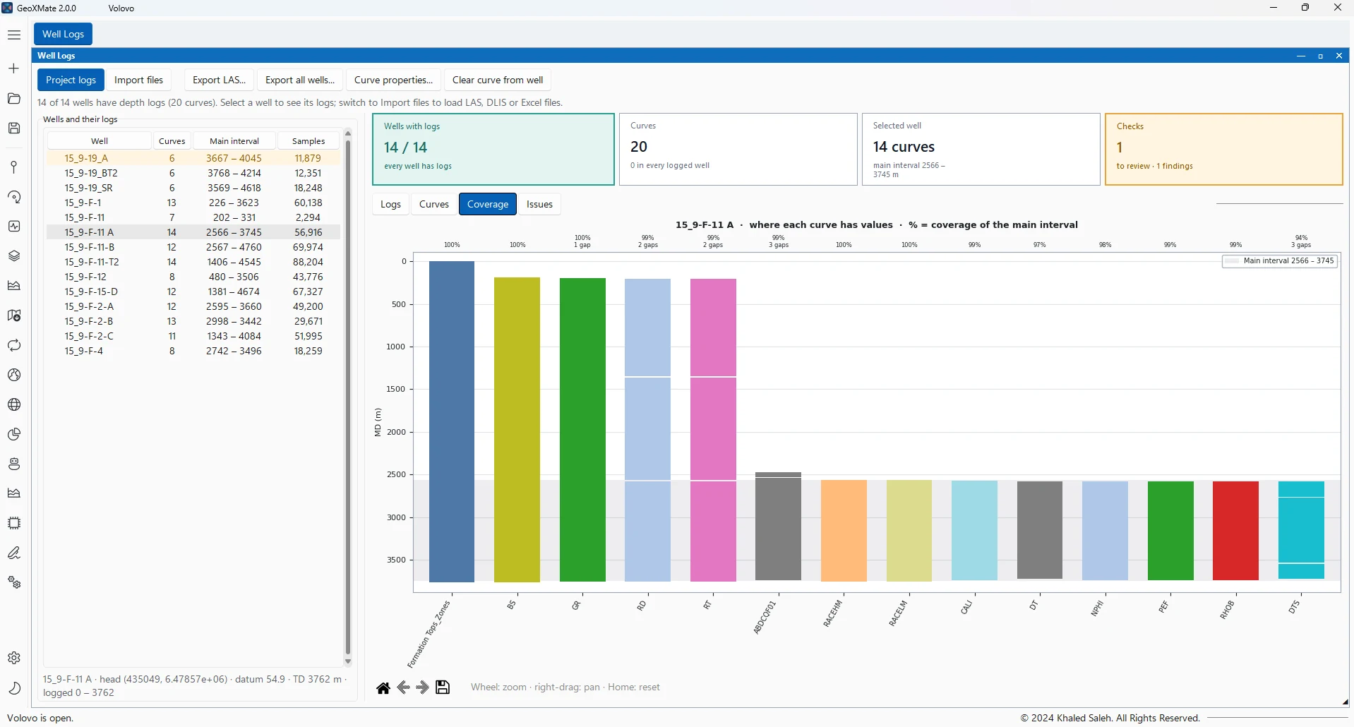
Every well's curves at a glance, with the coverage of each curve along the well and the issues to review.

Data	Formats	On import
Well headers	CSV, TXT, Excel	Columns recognised by name; duplicate names, shared heads, coordinates far from the field and missing datums are flagged before import. Latitude and longitude in decimal or degrees-minutes-seconds.
Well logs	LAS, DLIS, Excel	DLIS frames and Excel sheets are listed before reading; a sheet with a well column is split per well. Curves are matched to the project's existing logs.
Deviation surveys	Petrel and text traces, Excel	Converted to well paths by minimum curvature; TVD, TVDSS and X / Y along the hole.
Formation tops	CSV, TXT, Excel	Organised in sequences; an optional two-way time per top builds a time-depth relationship.
Time-depth relationships	Check-shot files, time logs, sonic	Calibrated by synthetic well ties; used to place wells on time seismic and to convert between domains.
Seismic cubes	SEG-Y (time or depth)	Indexed once and read in place, or converted to a compressed cube for fast access; cropped by lines, polygon or around wells.
Horizons	Petrel, CPS-3, ZMap+, IRAP classic, Earthvision, GOCAD, Charisma, IESX, column files	Points, grids and triangulated surfaces placed on the survey's bins; format recognised from the content.
Faults	Petrel, CPS-3, Landmark, Charisma, GOCAD, ZMap+, column files	Read as fault sticks and placed on the survey, one fault set per fault.
Maps	ZMap+ grids, X / Y / Z points	Point files are gridded on import; depth, time and velocity maps.
Geological models	Eclipse EGRID, GRDECL	Corner-point grids with zones, faults and all their properties.

Units

One set of units for the whole project

Logs, surveys, tops, seismic, horizons, maps and grids share the same coordinates and depth reference. A dataset drawn from several sources needs no further conversion before training.

Project units for X / Y, depth, time, velocity, area and volume
Each import asks for the item's own units and converts once, at the door
Seismic files are never rewritten: their axes are rescaled as they are read
Units are locked once data depends on them

Data transformation

New information from the data you already have

Derived curves are written beside the originals and never replace them, so the raw measurements stay available for comparison and for later models.

Log calculator: formulas over curves, such as logarithms, normalisations and cut-offs, previewed before writing
Encoder: discrete or text logs turned into class codes for training
Distance logs: the distance of every sample to a reference location
Time-depth conversion of logs, horizons and seismic cubes through well ties and velocity models
Seismic attributes and trace-to-log: the seismic along each well saved as new logs
Interpreted horizons and faults, picked in GeoXMate or imported

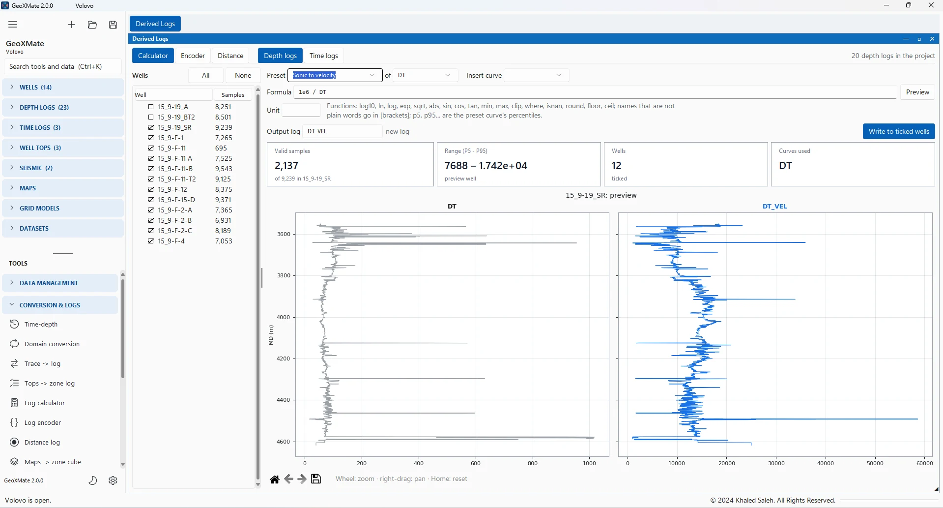
The log calculator: a sonic-to-velocity formula previewed on one well before it is written to the ticked wells.

Zone logs & zone cubes

Stratigraphy as an input to the model

Formation tops and mapped surfaces describe where a sample sits in the stratigraphy. Turned into logs and cubes, they become features a model can learn from, in wells and in 3D.

Zone logs: every log sample receives the code of the zone it falls in, from the formation tops
Zone cubes: an ordered list of maps or horizons divides the seismic survey into zones in 3D
Crossing surfaces are flagged in the preview before the cube is built
Zone cubes feed 3D prediction and can be exported to SEG-Y

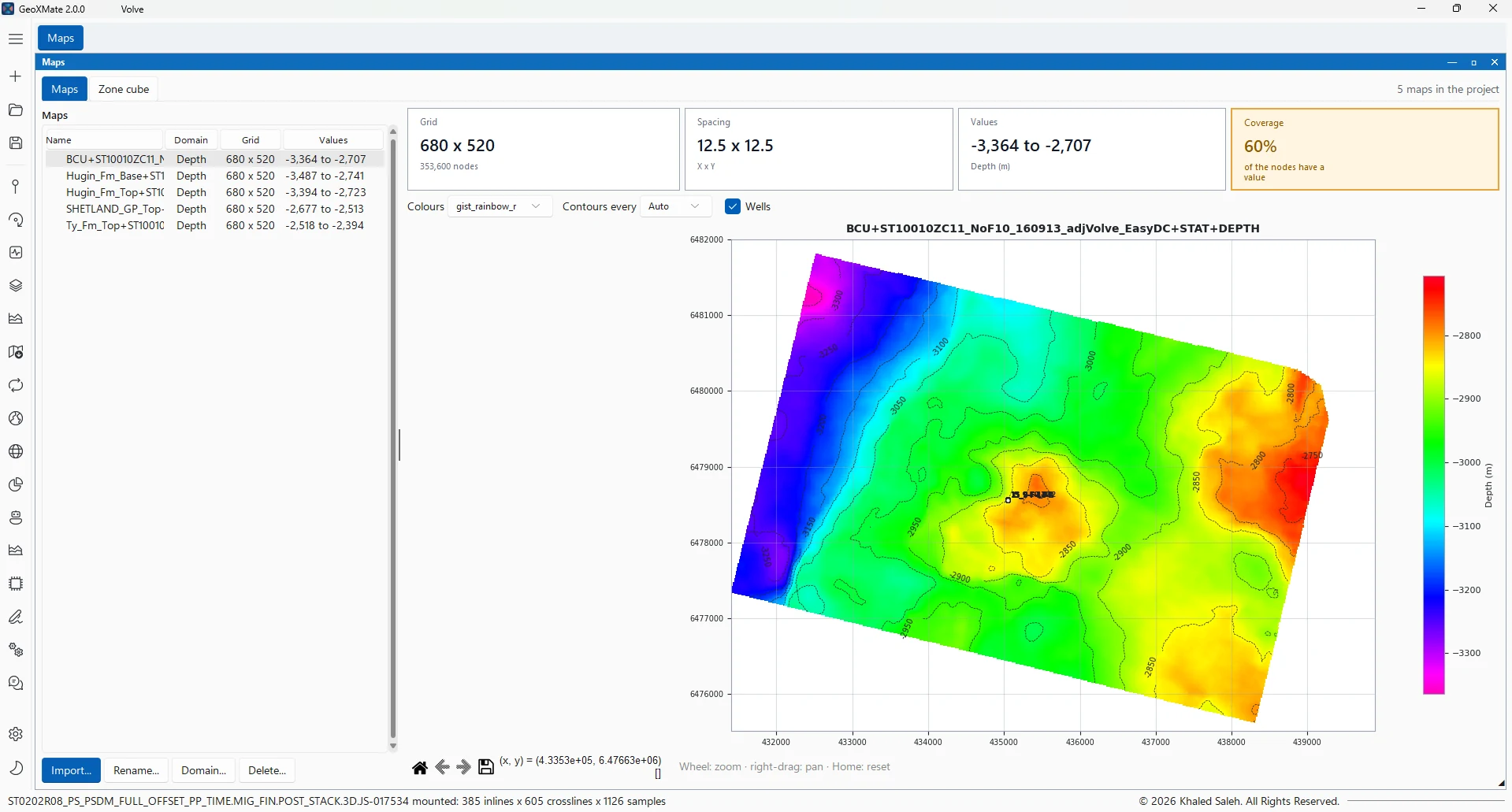
The base Cretaceous depth map with its contours and the wells, one of five surfaces that the Zone cube tab turns into zones in 3D.

Smart correlation

Well correlation with assisted top picking

The correlation panel shows wells side by side in TVDSS or MD, with zone columns, log tracks and the zones filled between wells. While the geoscientist picks, GeoXMate proposes where the active top should be in each well and says how confident it is.

Interpreter-guided

Assisted top picking

A reference well's picks are carried to the other wells by matching the logs around each top, checked against the structure and the thickness of the nearest wells.

How it works

The logs are compared as robust z-scores, resistivity on a logarithmic scale, so different tools and vintages line up.
A window around the reference pick is slid and stretched (0.8 to 1.25 times) along the target well; the best correlation marks the candidate depth.
Independent estimates from a plane through the nearest wells' picks and from the zone thickness check the candidate.
Each proposal is rated High, Medium or Low confidence; a hover guide shows the match anywhere along the well.

ResultStaged picks the geoscientist accepts or moves, saved in the tops sequence with their measured depth from the survey.

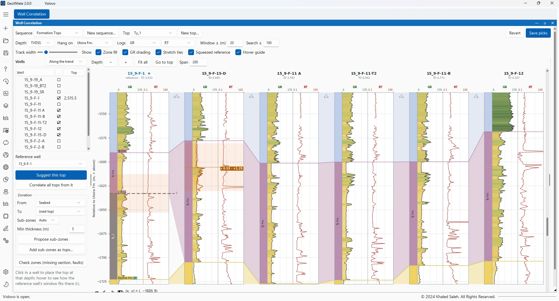
Assisted picking: the reference well's window found in the next well, with its correlation and stretch (r 0.53, x1.25).

Interpreter-guided

Sub-zones and Zone QC

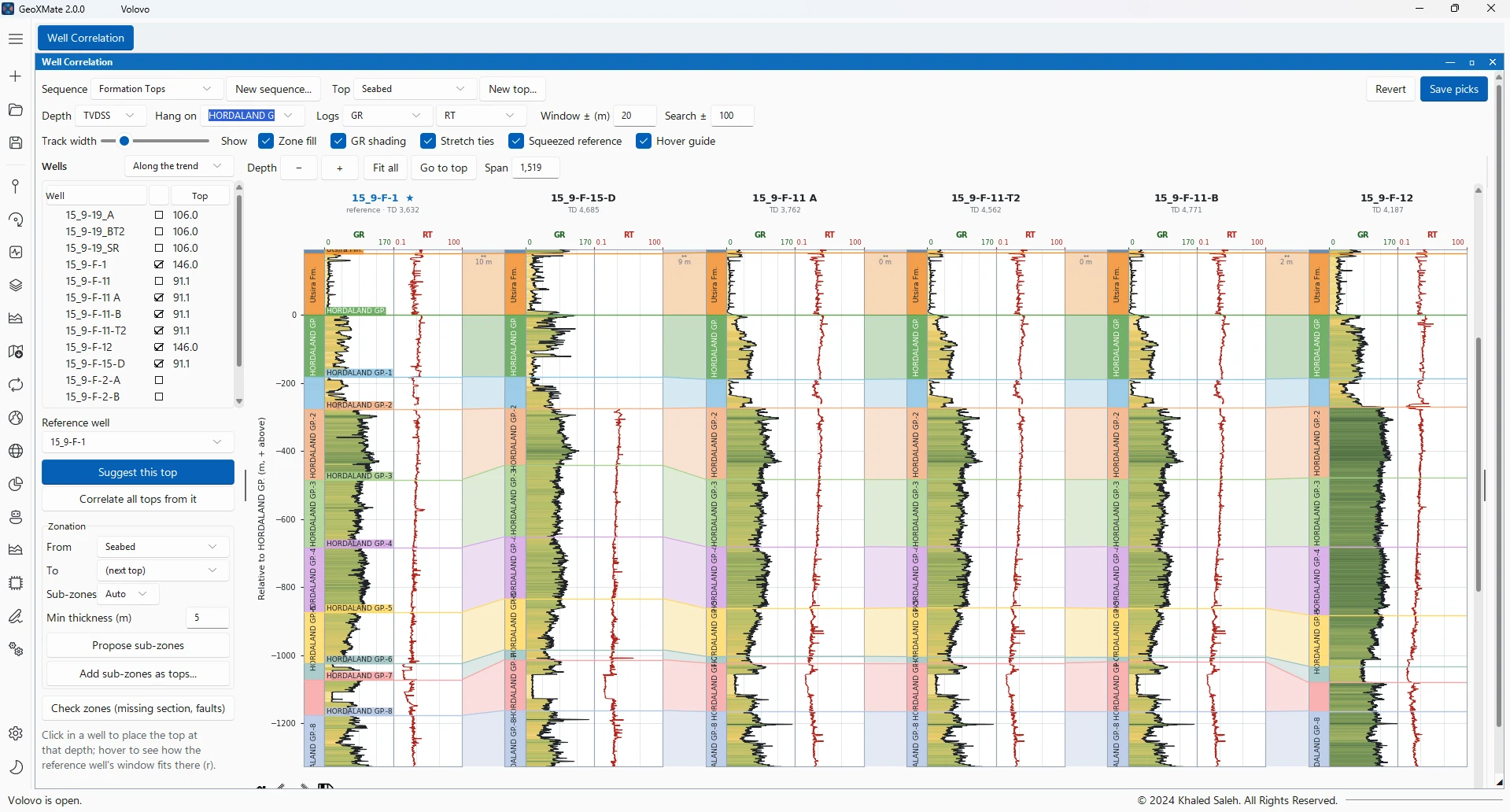
Between two tops picked in both wells, the logs are aligned sample by sample to find sub-zones and sections that are missing or repeated.

How it works

Sub-zones are proposed in the reference well by segmenting its logs, then carried to each well by dynamic time warping.
A sub-zone that thins out is marked as missing; each sub-zone's stretch factor is shown between the wells.
Zone QC compares the zone's thickness with the nearest wells and flags structural steps of two tops or more.

ResultSub-zone tops and quality flags that can be written as zone logs and used as training labels or features.

Sub-zones of the Hordaland Group carried across six wells, flattened on the top of the group.

Next: from data to a dataset

Select wells, logs and zones, then inspect, clean and train.

The machine-learning workflow