3D geological models

Geological models populated by geostatistics and machine learning

GeoXMate works on the cells of corner-point geological models, imported or built in the project. Alongside the conventional modelling workflow, properties can be distributed with machine learning, using the seismic and the model's own geometry as inputs.

Structural model

Import a model or build one from maps and faults

  • Eclipse EGRID and GRDECL models imported with all their properties, converted to the project's units
  • New models built from depth maps and fault sticks, with the layering set per zone
  • Geometry and QC: cell volume, height, angle, twist, inside-out and negative-thickness cells, rated against limits saved with the model
  • A 3D view of the whole model, slices along I, J and K, fences and boxes
  • Imported properties are never overwritten by calculated geometry
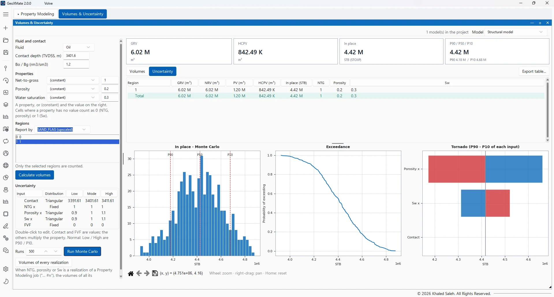
The Volve structural model in 3D: 41,280 active cells coloured by layer, with 20 wells and their formation tops.

Upscaling

Well logs into the cells

  • The samples of each well are placed in the cells its path crosses and averaged per cell
  • Continuous logs, facies and zone logs, each with the averaging that suits it
  • The upscaled cells are the conditioning data for geostatistical modelling and the training data for machine learning
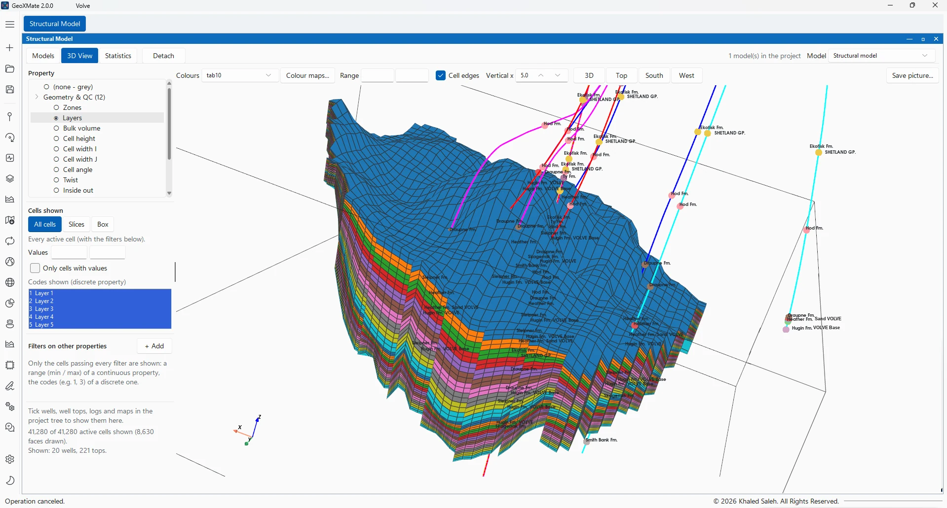
The sand flag upscaled from the wells: only the 306 cells the well paths cross receive a value.
MethodTypical use
ArithmeticPorosity, saturation, net-to-gross
HarmonicFlow across layers, such as vertical permeability
GeometricRandomly arranged values, such as horizontal permeability of mixed rocks
RMS, median, minimum, maximumOther continuous logs
Most ofFacies and zones: the most frequent code in the cell

Seismic resampling

The seismic in every cell

Wells sample a few hundred cells; the seismic covers the whole model. Resampling the cube into the grid carries that lateral information into property modelling.

  • A seismic cube or attribute read at every active cell, not only where the wells are
  • Sampled at the cell centre, or averaged over the cell's height
  • Depth cubes read directly; time cubes through a time-depth relationship
  • The resampled property guides co-kriging and co-simulation, and is an input to machine-learning modelling
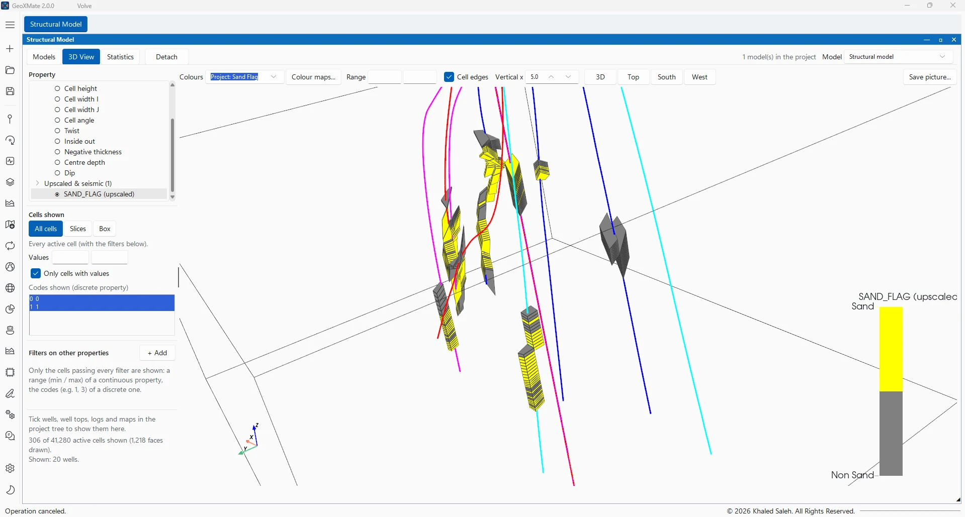
The depth seismic cube resampled into all 41,280 cells, ready to use as an input for property modelling.

Property modelling

Conventional facies and property distribution

  • Data analysis per zone and facies: transforms, variograms with auto-fit, vertical proportion curves and trends
  • A modelling method per zone, with its variogram from the data analysis
  • Continuous properties modelled per facies from their own data
  • Simulations run in parallel, zone by zone
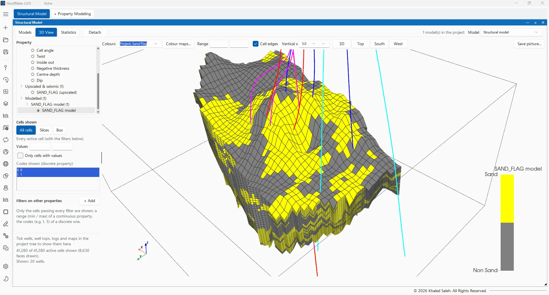
The upscaled sand flag distributed through every cell of the model: sand in yellow, non-sand in grey.
PropertiesMethods
Continuous propertiesSimple and ordinary kriging, Gaussian simulation (SGS), inverse distance, nearest, constant value
FaciesIndicator simulation (SIS), indicator kriging, nearest, most common code
Secondary dataCo-kriging and co-simulation with a correlated property, such as a seismic attribute
UncertaintySeveral realisations with their mean, P10, P50 and P90, or the probability of each facies

Machine-learning modelling

Properties predicted in every cell

Machine learning brings the seismic, the zones and the position of each cell into the distribution of a property. Three routes are available, with the same validation principle as in wells: whole parts of the model are held out to measure the result.

Supervised ML

Train on the cells

A property known in the cells the wells cross, such as an upscaled log or facies, is learnt from the other properties of those cells and predicted in every active cell.

How it works
  1. Inputs are any properties of the model: seismic resampled into the cells, attributes, zones, depth and position.
  2. Any of GeoXMate's classification or regression algorithms can be chosen.
  3. Blocks of columns are held out for validation, since neighbouring cells are nearly copies of each other.

ResultA new property in every active cell, with its validation score.
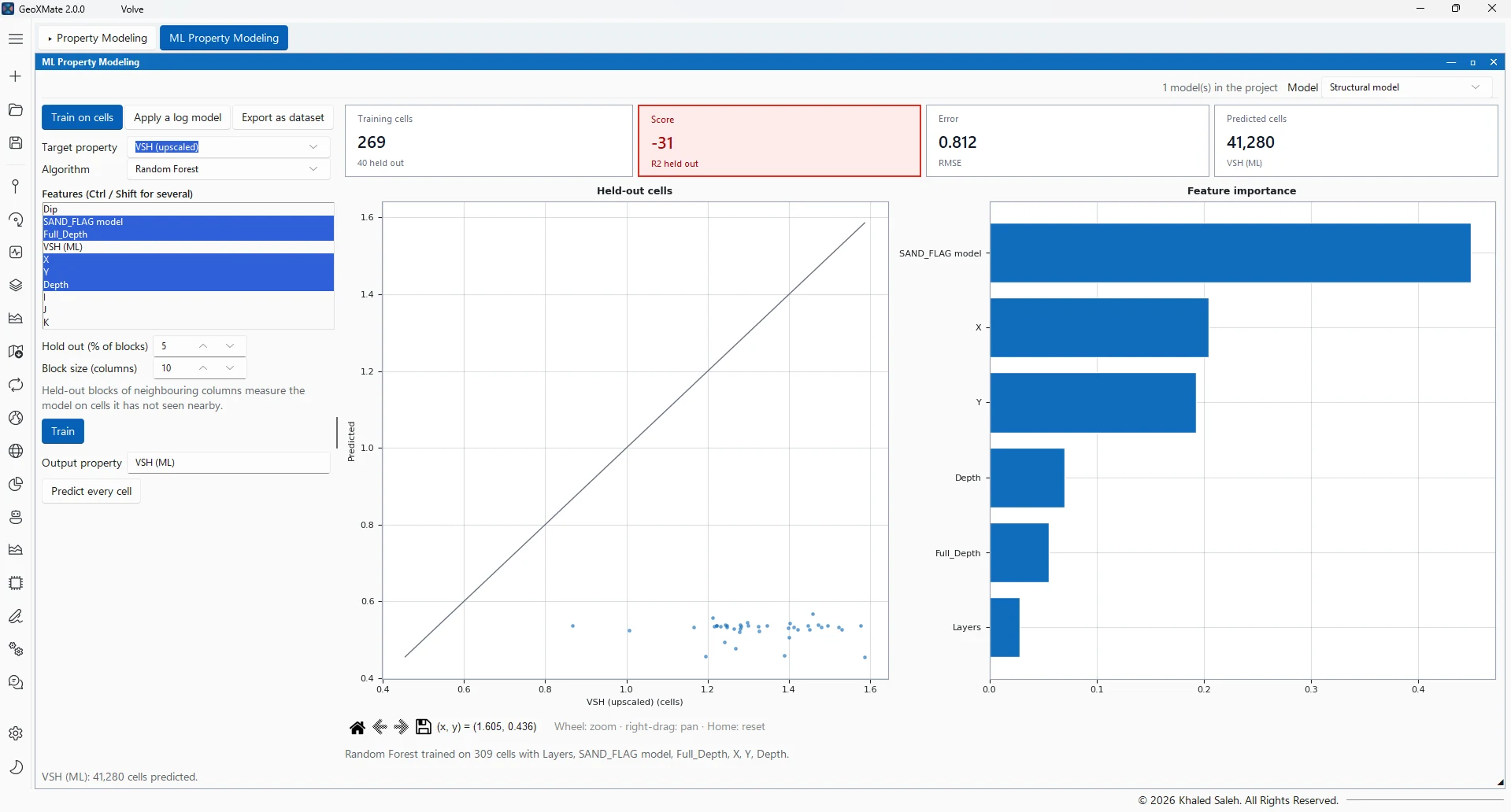
A Random Forest trained on the cells predicts shale volume from the sand model, the seismic, X, Y and depth, scored on held-out blocks of columns.
Supervised ML

Apply a model trained on wells

A model already trained and evaluated on well logs runs on the cells, each of its input logs matched to a property of the model.

How it works
  1. The model is chosen from the project's saved classification or regression models.
  2. Each input log is matched to a model property with the same meaning, such as an upscaled or seismic-derived property.
  3. Cells whose inputs lie outside the training range can be left empty.

ResultThe well-log model's prediction in every cell, consistent with what was evaluated in the wells.

Supervised ML

3D datasets and deep learning

The cells of a model become a dataset in their own right, for the Data Explorer and the machine-learning tools, or 3D patches for deep-learning networks.

How it works
  1. Cells are exported as a dataset, with each block of columns treated as a well and the cell centre as its depth.
  2. The full workflow then applies: visualization, cleaning, comparison, feature selection, tuning and evaluation.
  3. For 3D networks, the model's properties are read as patches around wells or across the area, and the network's answer is written back as properties.

ResultModels trained on the geological model itself, with every tool of the machine-learning workflow.

Volumes

In-place volumes and their uncertainty

  • Gross rock, net rock, pore and hydrocarbon pore volumes by zone or segment
  • Oil and gas in place in stock-tank barrels and standard cubic feet
  • Monte Carlo on the contact, net-to-gross, porosity, saturation and formation volume factor
  • P90, P50 and P10, histogram, exceedance curve and tornado chart
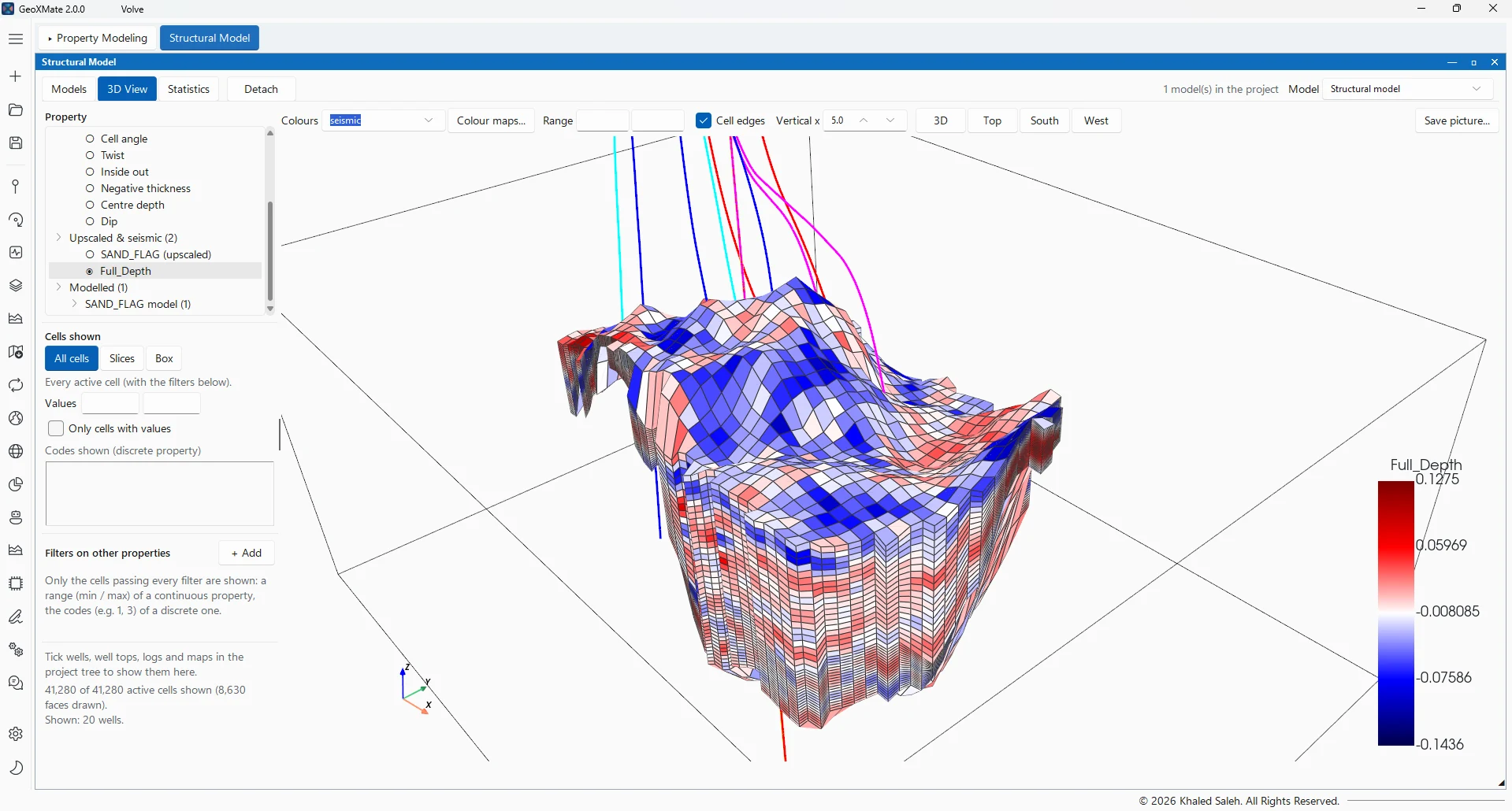
Oil in place from 500 Monte Carlo runs on the contact, porosity and saturation: P50 4.42 million STB (P90 4.18, P10 4.68), with the exceedance curve and the tornado chart.