Machine learning
The whole machine-learning workflow, without code
GeoXMate gives the geoscientist a tool for each stage of model development, from the first look at the data to the application of the final model. Every stage validates by well, so the decisions made along the way are judged the same way the final model will be.
Datasets
A dataset is the starting point of every model
Datasets are saved in the project. The project's well data is never changed by what happens to a dataset, so several datasets can be cleaned and compared side by side.
- Select wells, logs and zones from the project, in depth or in time
- Logs from different sources: measured, derived, zone logs, seismic along the well
- Dataset details: rows, wells, logs, complete rows, coverage and per-log statistics
- Datasets can also come from the cells of a geological model
Visualization
Understand the data before training on it
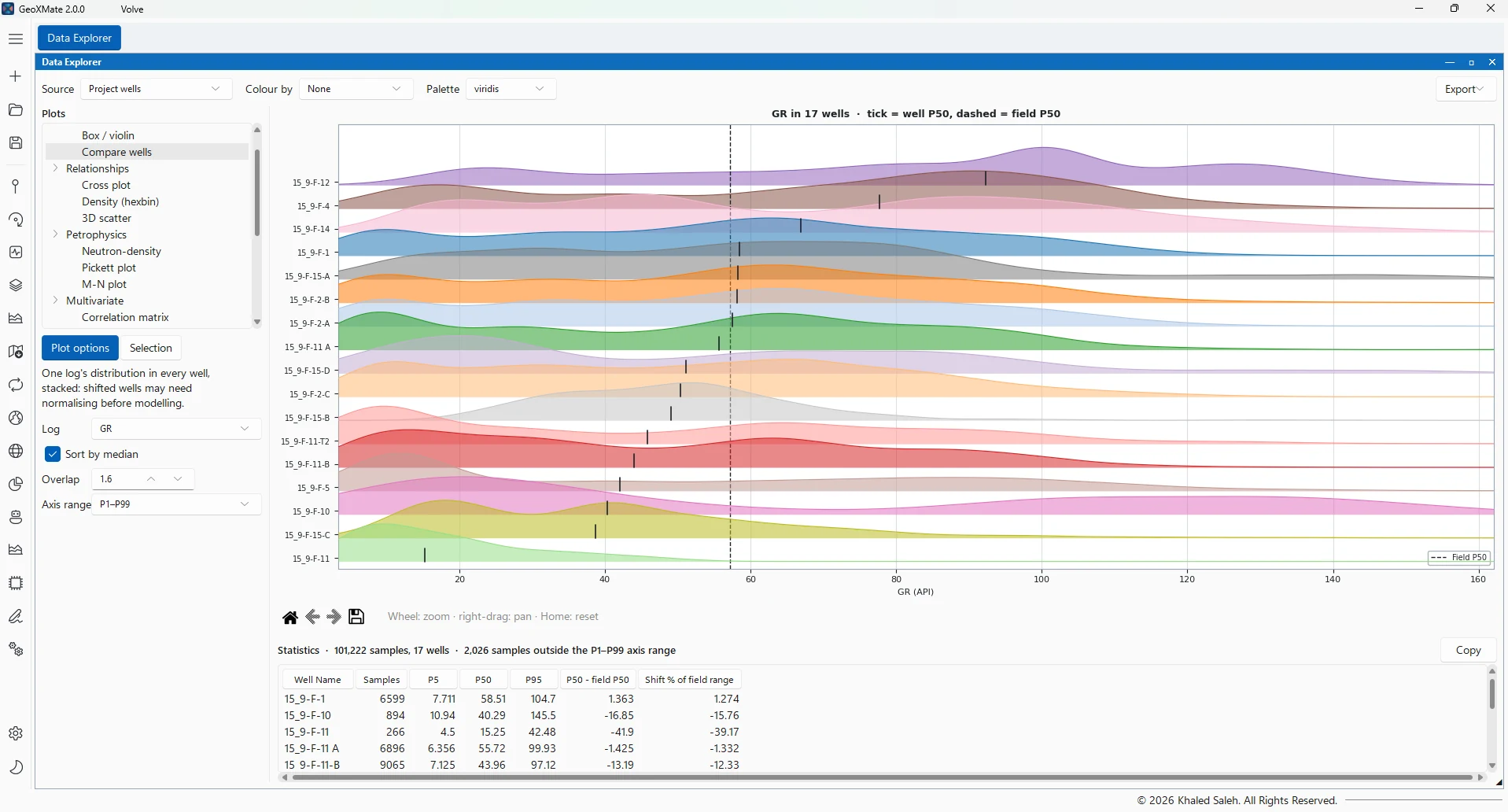
Charts show the distribution of each log, the relationships between logs, how the wells differ and where the outliers are, so the cleaning that follows is based on evidence.
- One Data Explorer for every analysis chart, on a dataset or straight on the wells
- One selection of wells, depth window and classes applies to every chart
- Colour by any log, well or class, with the project's facies colours
- Statistics of the current selection under every chart, ready to copy
Distributions
Relationships
Petrophysical
Wells and depth
Feature insight
QC & cleaning
Find the problems, fix them in a recipe
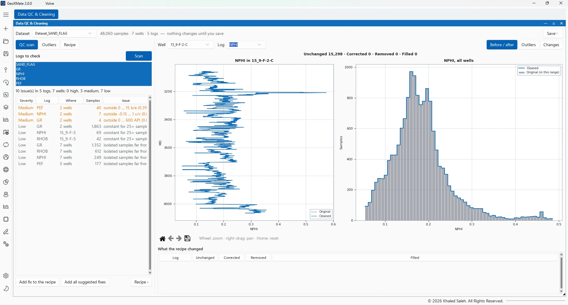
- A QC scan lists the problems in the data, most severe first, each with a suggested fix
- Fixes are steps of a recipe, applied to the original samples, never in place
- Any step can be edited, reordered or removed, and the result is recomputed
- A before-and-after view shows what each step changed, per log and per well
- The cleaned data is saved as a new dataset for training
What the scan finds
Recipe steps
| Outlier removal | Methods |
|---|---|
| Univariate | IQR (Tukey fences), Z-score, modified Z-score (MAD), percentiles |
| Multivariate | Isolation Forest, Local Outlier Factor, robust Mahalanobis distance |
| Scope and action | Per well or over the whole dataset; blank the values or drop the rows |
Training
Classification and regression with a wide range of algorithms
Algorithms are grouped by family; each family covers both classification and regression, and every algorithm is available in every tool: training, comparison, feature selection, tuning and evaluation.
- Classification for facies, lithology and zones; regression for continuous logs and properties
- Training, test and leave-one-well-out wells chosen in the same validation panel
- Class balancing (SMOTE) applied to the training rows only
- Every model saved with its inputs, settings and validation scores
| Family | Algorithms |
|---|---|
| Tree ensembles and boosting | Random Forest, Extra Trees, Decision Tree, Histogram Gradient Boosting, XGBoost, LightGBM, CatBoost |
| Linear | Logistic Regression, Ridge Classifier; Linear, Ridge, Lasso and Elastic Net regression |
| Kernel and distance | K-nearest neighbours, Support Vector Machine, Gaussian Process; SVR and Kernel Ridge |
| Neural networks | Dense neural networks (Neural Network add-on) |
| 3D deep learning | CNN 3D, ResNet 3D, U-Net 3D, Bi-LSTM on seismic and grid patches (Deep Learning add-on) |
Optimisation
Find the best model, the best inputs and the best settings
Three optimisation tools work on the same validation by well, so every comparison is fair and every gain is measured on wells the model did not learn from.
Which algorithm suits this data
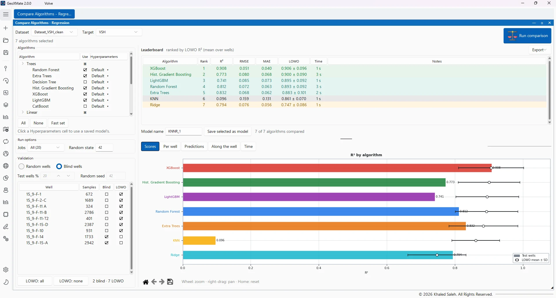
Several algorithms are trained on the same wells and ranked in a leaderboard by accuracy, balanced accuracy or macro F1, R² or RMSE, the leave-one-well-out mean and the training time. Results can be viewed per well, as predictions and along the well.
Which logs the model needs
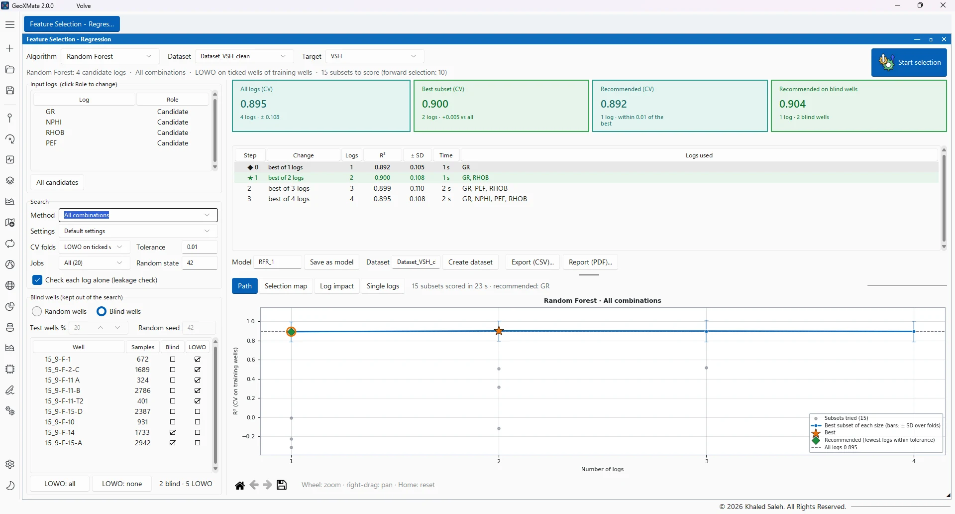
Backward elimination, forward selection or importance ranking find the subset of input logs that scores best. A leakage check flags a single log that predicts the target almost alone. The recommended subset is confirmed on blind wells.
How the model should be set
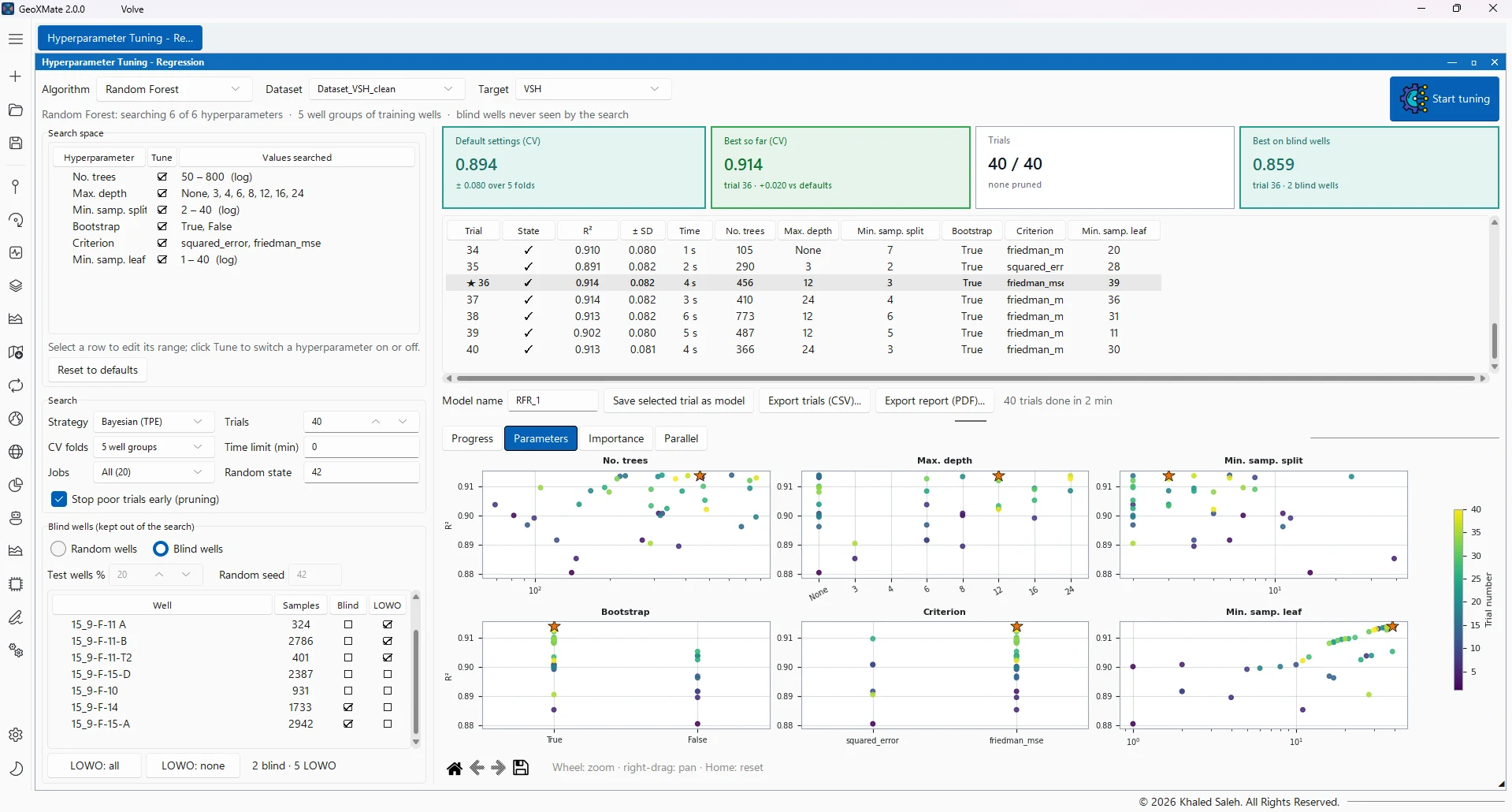
A Bayesian (TPE) or random search explores each algorithm's settings, with unpromising trials stopped early. Every trial is scored by well, and the best settings train the final model.
Evaluation
Judged on wells the model has never seen
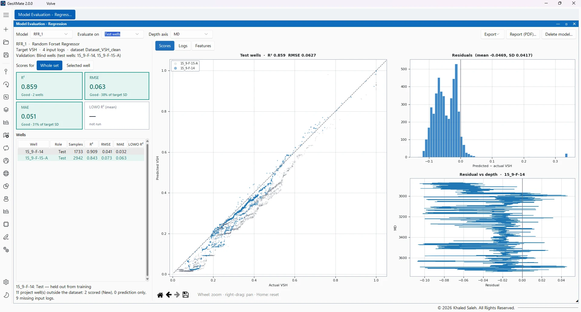
Samples from the same well are strongly related, so a random split of rows overstates any model. GeoXMate always holds out whole wells. A model's result is trusted only when it is scored on wells held out of training.
- Blind wells: chosen wells are kept out of training and of every feature search
- Leave-one-well-out (LOWO): each ticked well is predicted by a model trained without it
- Random test wells: a share of the wells is held out at random, never a share of the rows
- New wells outside the dataset are scored too, wherever their logs allow
| Models | Evaluation tools |
|---|---|
| Regression | R², RMSE, MAE per well and pooled; predicted against measured crossplot; residual histogram; residuals against depth; predicted and measured logs along each well |
| Classification | Accuracy, balanced accuracy, macro F1; confusion matrix; precision, recall and F1 per class; predicted and true class proportions; original, predicted and match tracks along each well |
| Every model | Scores per well with each well's role (held out, training, new); a rating of the score; feature importance by permutation or SHAP |
Application
Apply the model where the data is
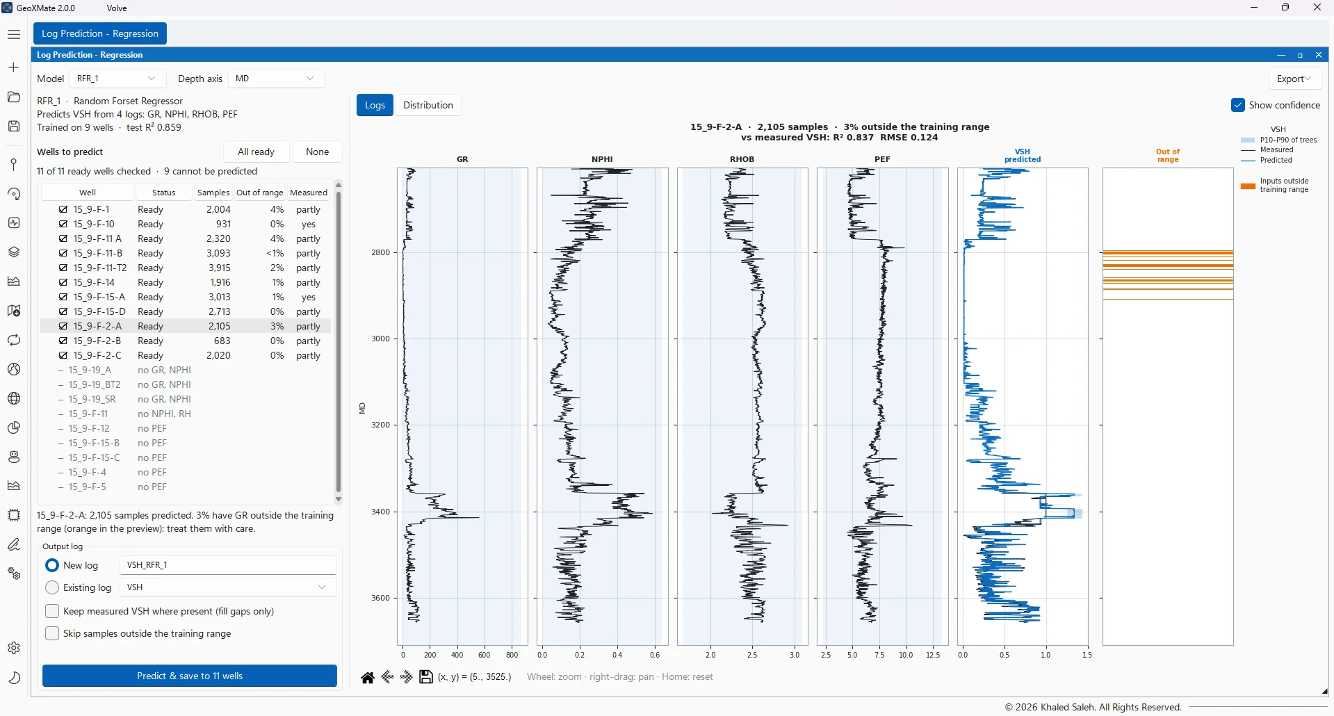
A trained model is applied in wells, in seismic volumes and in geological models through the same code path, so the prediction matches what was evaluated.
- Log prediction on any number of wells, with the inputs each well is missing listed
- Samples outside the training range marked, with a confidence measure where the model has one
- Prediction onto a seismic cube, with attributes computed on the fly, and class probabilities
- Prediction into the cells of a 3D geological model