3D seismic

Seismic interpretation with machine learning

GeoXMate offers each interpretation task in more than one way: guided by the interpreter, learnt from the interpreter's own picks, or found in the seismic without any labels. The methods share the same survey, the same interpretation store and the same views, so their results can be compared on the same section.

Seismic data

The seismic volume as a source of training data

Seismic attributes are computed as cubes or on the fly along the wells and during prediction, so a model trained on an attribute can be applied to the whole survey without storing it first.

SEG-Y cubes in time or depth, read in place or converted to a compressed cube for speed
Inline, crossline and time-slice views with wells, tops, horizons and faults; a 3D view of all of them
Cube insights: coverage, amplitude distribution, frequency spectrum and phase
Synthetic well ties, wavelet extraction, velocity models and domain conversion
Trace to log: amplitudes, attributes or other cubes along each well, saved as logs for 1D datasets

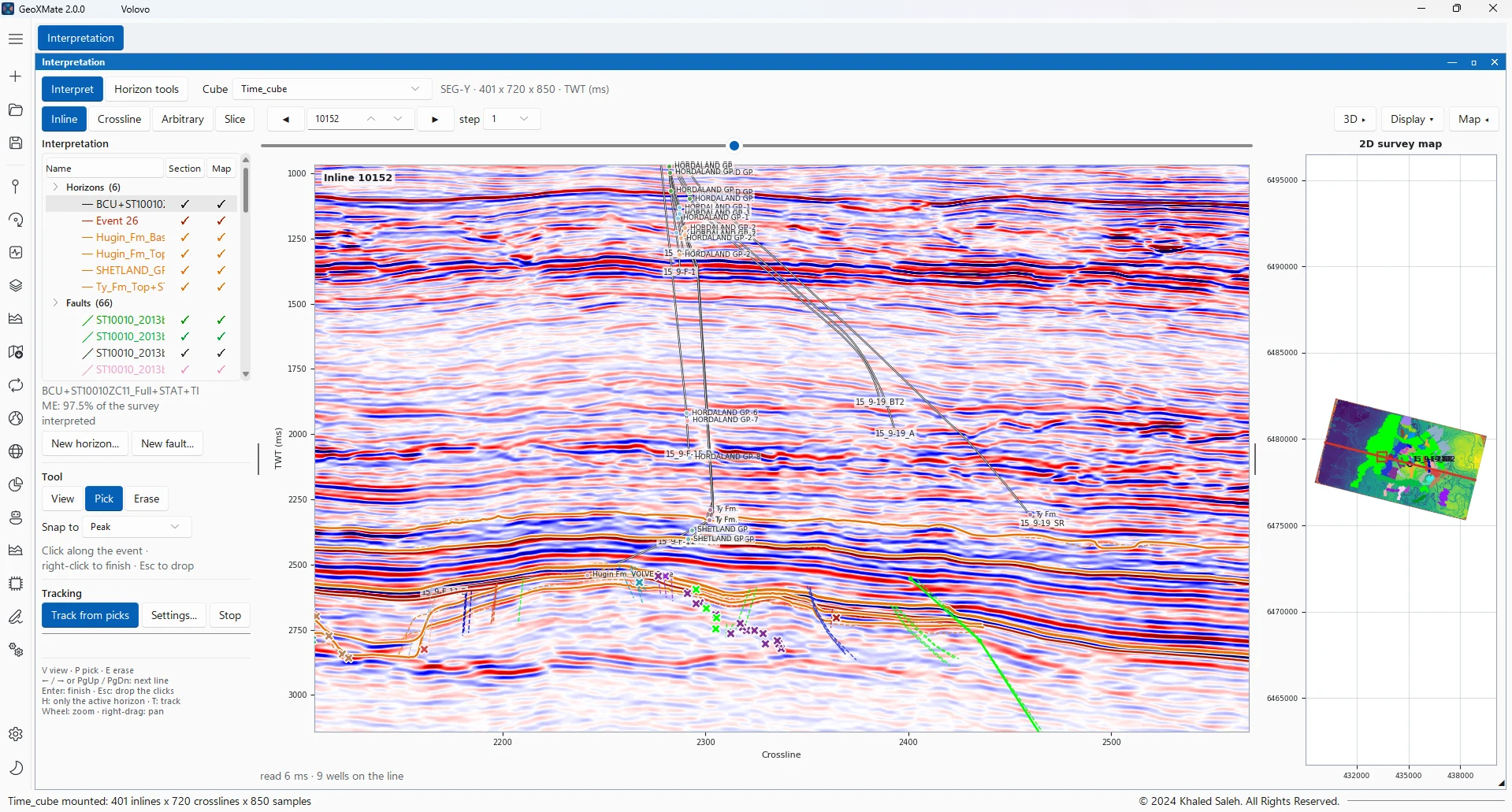
An inline of the Volve cube with wells, formation tops, interpreted horizons and fault sticks, beside the survey map.

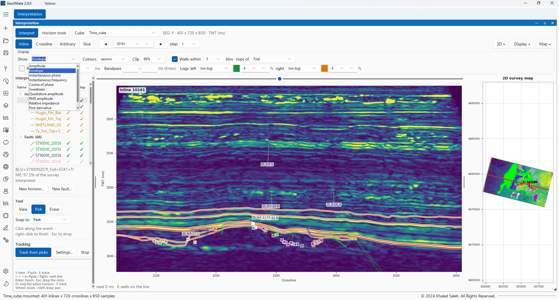
The envelope attribute computed on the fly on an inline, with the list of attributes open.

Seismic attributes

EnvelopeInstantaneous phaseInstantaneous frequencyCosine of phaseSweetnessRMS amplitudeAGCBandpassSpectral decompositionRelative impedanceCoherenceFault planarity lossFault dip changeFault energy change

Horizon interpretation

Three ways to interpret horizons

From classic seeded tracking to a network trained on the interpreter's lines and an unsupervised reading of every reflection in the cube.

Interpreter-guided

Guided picking and tracking

The interpreter places a few picks; GeoXMate follows the event between them and grows the horizon across the survey.

How it works

Between two clicks on a section, the event is followed along the best path through the seismic, weighing event strength and waveform likeness.
Tracking grows the horizon from all picks to neighbouring bins that hold the same event, look alike and agree with their picked neighbours, most similar bins first.
Fault sticks act as barriers that the growth does not cross.
A quick frame can be tracked along every n-th line first, then filled between the lines.
The misfit against the well tops is measured, and a copy corrected to them can be saved.

ResultA horizon on the survey's bins, shown on any cube of the same survey and ready for maps, zone cubes and models.

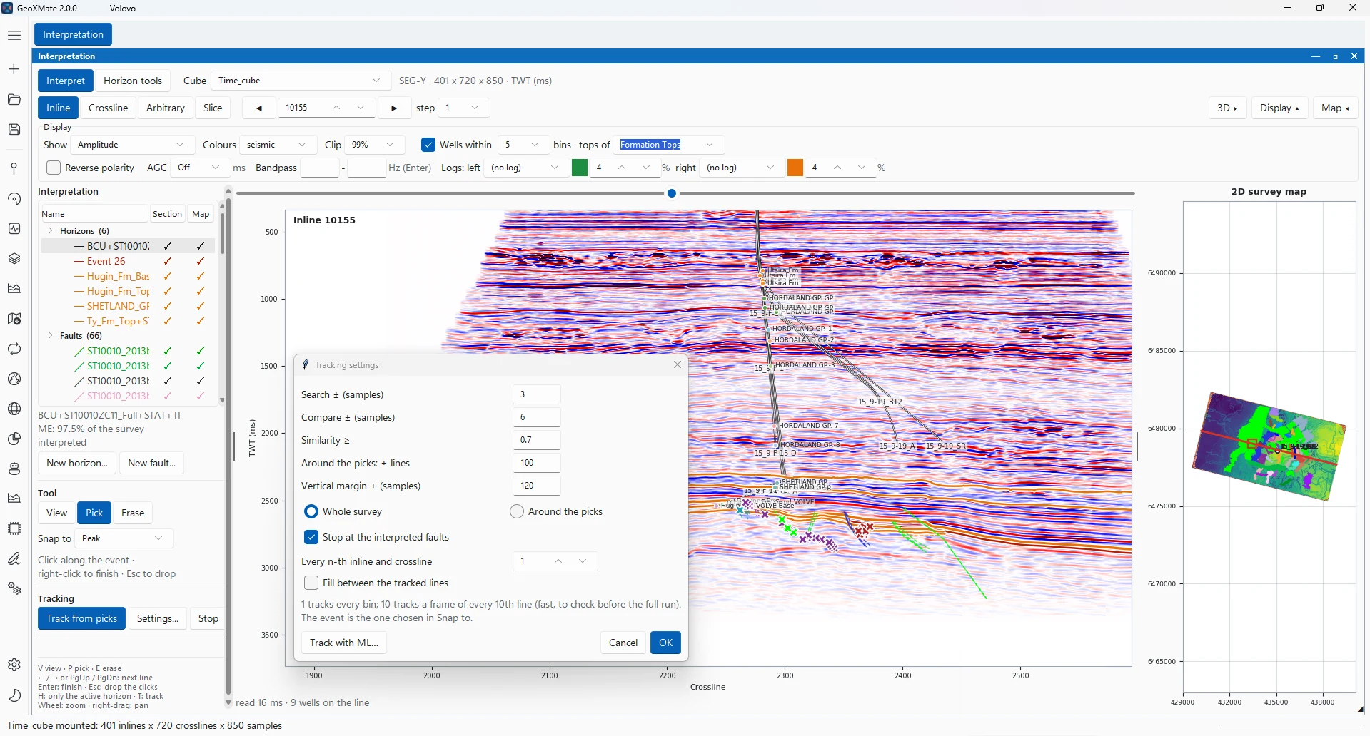
Tracking settings: search and comparison windows, the similarity threshold, and the interpreted faults as barriers.

Supervised ML

ML Horizon Tracking

A neural network learns how the interpreter follows a horizon on a few interpreted lines, then tracks it over the whole survey.

How it works

A prior surface, interpolated from the picks between guide horizons, centres a search window on every trace.
Training patches are cut around the picked traces; whole interpreted lines are held out as blind lines.
A U-Net 3D or Bi-LSTM network predicts the horizon's position along each trace in the window.
The blind lines measure the error (mean, P90, share within one and two samples) beside the prior and the classic tracker.
The surface grows from all picks over the network's candidates, respecting guide horizons and fault barriers.

ResultA horizon with a confidence value per trace, measured against the interpreter's own blind lines.

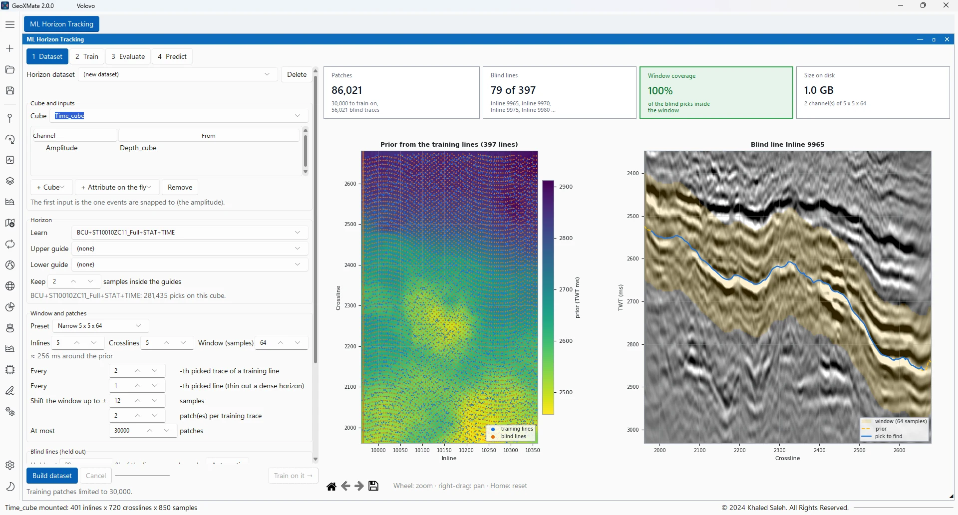
The training dataset: the prior from 397 training lines, and a blind line with the window the network searches.

Unsupervised ML

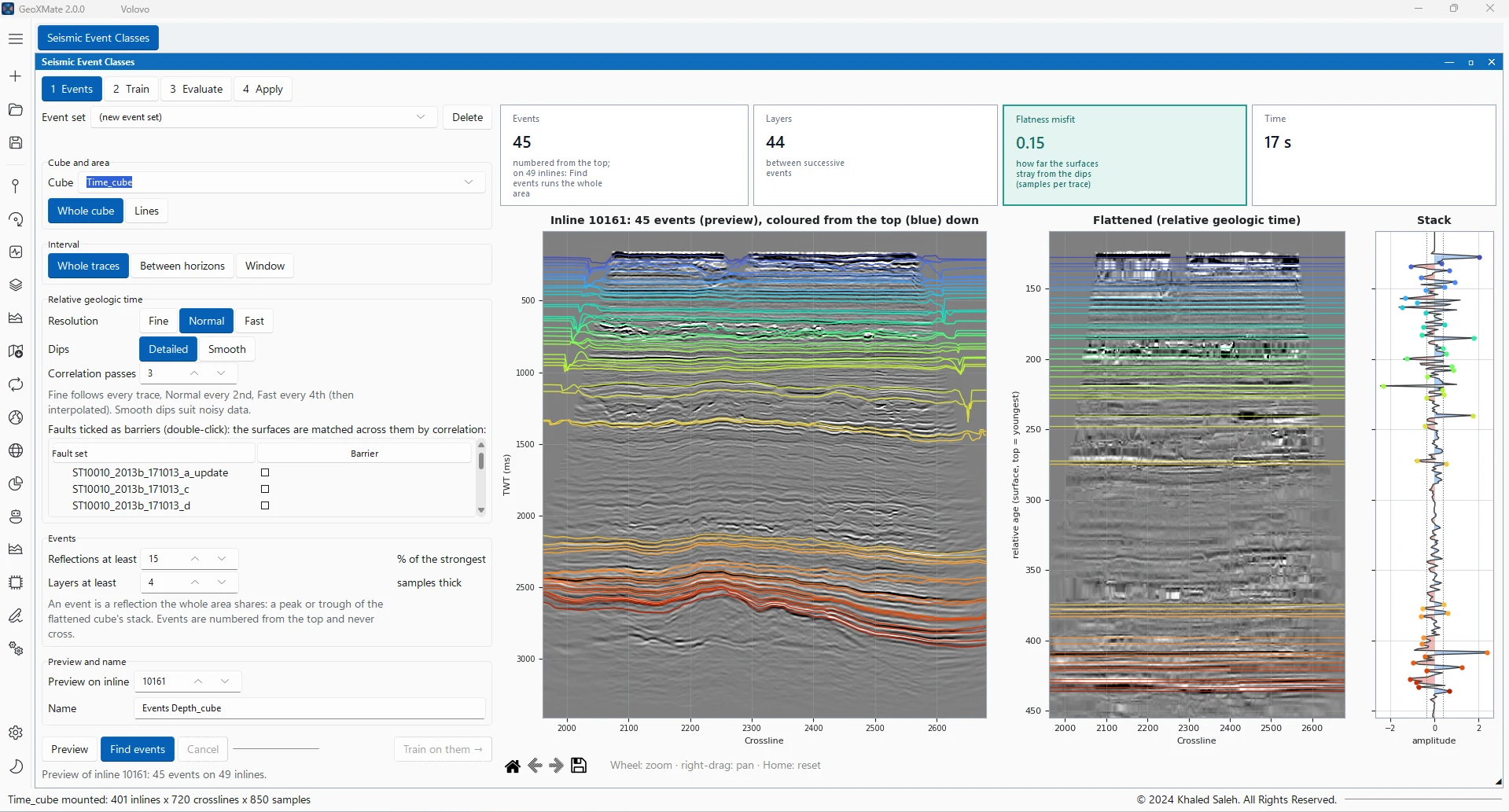
Seismic Event Classes

Every reflection in the cube is followed as a surface of relative geologic time; the layers between the main events are then grouped into seismic facies classes without labels.

How it works

Local dips are measured with the structure tensor, weighted towards strong, continuous reflections.
One surface is fitted to the dips at every sample; surfaces may touch at onlaps and pinch-outs but never cross.
Faults cut the surfaces, and the blocks either side are realigned by matching the flattened traces.
The main events are the peaks and troughs of the flattened cube; each layer between them is described by its thickness, amplitude, frequency, continuity, dip and roughness.
K-means or a Gaussian mixture groups the layers; the number of classes is recommended from the silhouette score and each class is described in words.

ResultA class map for every layer and a class cube, with sections, a flattened view, stratal slices and quality views to review them.

Forty-five events found on an inline, the section flattened to relative geologic time, and the stack the events come from.

Fault interpretation

Faults found with and without labels

Fault sticks can be picked, imported from other software, found in the seismic alone, or learnt from the interpreter's picks. Both machine-learning methods end in the same fault surfaces and probability cube.

Unsupervised ML

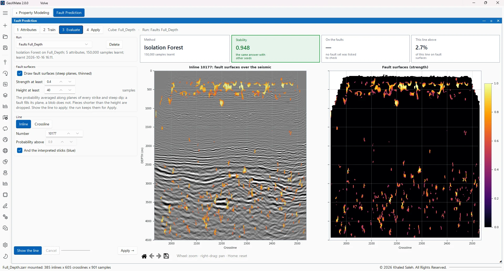
Unsupervised Fault Prediction

Faults are found from the seismic alone. Interpreted faults are used only to check the answer, never to train it.

How it works

Five fault attributes are computed: dip-steered discontinuity, planarity loss, dip change, curvature and energy change.
Each attribute is read against its own lateral background, so a noisy interval does not look like a fault.
An Isolation Forest, K-means or a Gaussian mixture scores how fault-like each sample is.
Planes of every strike and steep dip are scanned through the score; the best plane is kept, thinned and only tall connected pieces remain.
The result is checked against any interpreted fault sticks.

ResultA fault probability cube and fault surfaces, which can also serve as starter labels for the supervised method.

An Isolation Forest on five attributes of the depth cube, with no labels: fault surfaces over an inline, and a stability of 0.948 between seeds.

Supervised ML

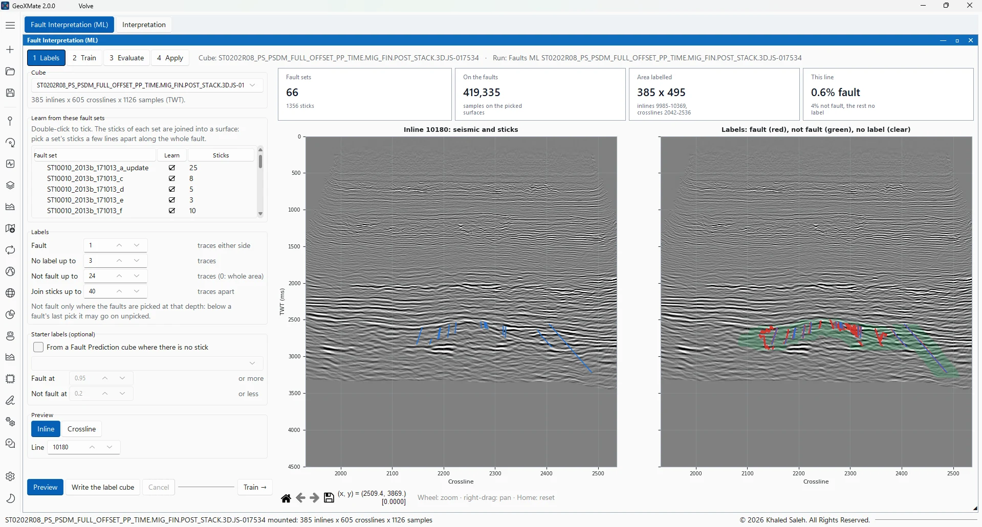
Supervised Fault Prediction

A model learns the faults from the interpreter's fault sticks and finds them, and the faults left unpicked, across the cube.

How it works

Each fault's sticks are joined into a surface.
Labels are set by the distance to the surface: fault close to it, no label in an uncertain band, not fault beyond, and only at the depths where faults were picked.
A U-Net 3D trains on the seismic balanced by its RMS amplitude; boosted trees on the fault attributes are offered without any add-on.
Whole blocks of the cube are held out to score the model on faults it did not see.

ResultA fault probability cube and fault surfaces in the interpreter's own style.

Labels from 66 interpreted fault sets: the sticks joined into surfaces, then fault in red, not fault in green and no label left clear.

3D deep learning

Networks that learn from the volume itself

Where a 1D dataset sees a well as a column of samples, a 3D dataset gives the network the seismic around each sample, so lateral changes in the reflections become part of what it learns.

3D datasets of patches around well samples, with a log as the target, or over the whole area, with a cube or property as the target
CNN 3D and ResNet 3D answer for the patch centre, Bi-LSTM along the centre trace, U-Net 3D for the whole patch
Held-out wells or blocks are never trained on nor used to stop training; scores come only from them
Runs on the GPU when one is available, with mixed precision; on the CPU when not
Predictions written as a new cube, with class probabilities, or as properties of a geological model

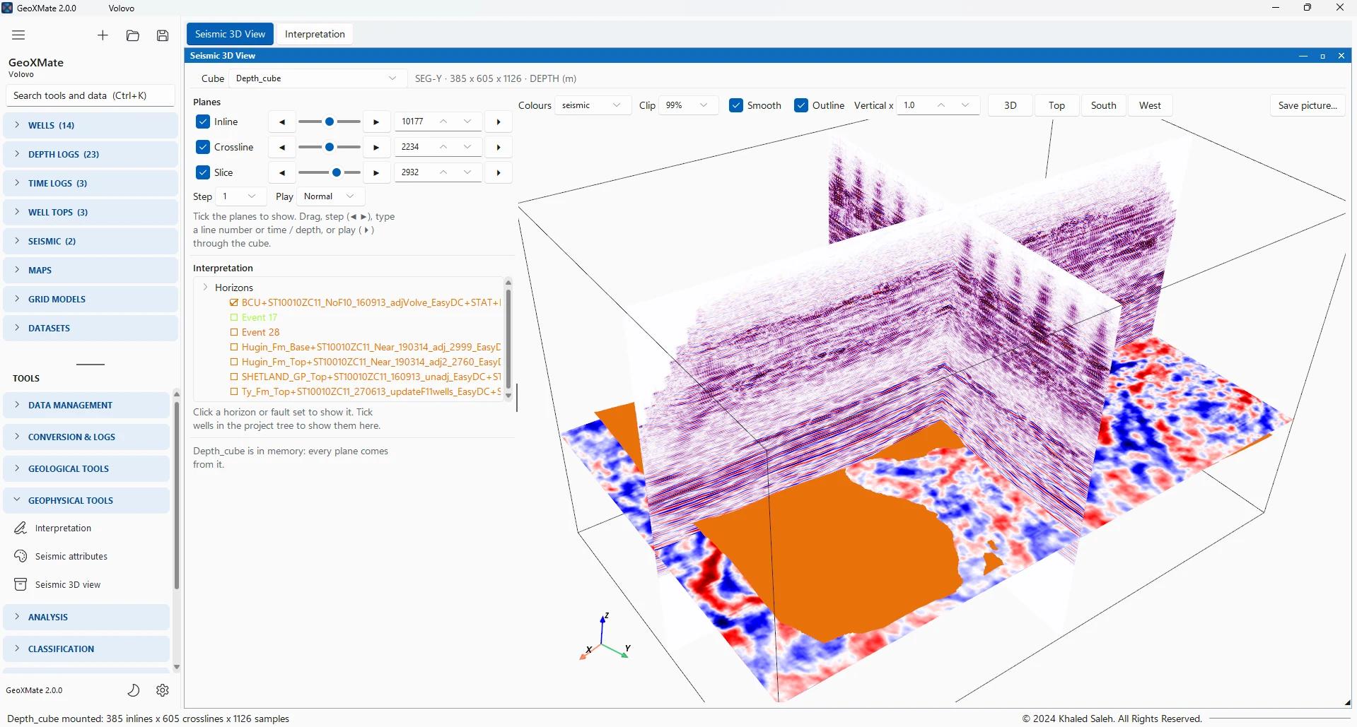
Inline, crossline and depth slice of the depth cube in one 3D scene, with an interpreted horizon.

Next: 3D geological models

Bring the seismic and the wells into the cells of a model.

3D geological modelling